Here is the procedures step-by-step

1. Build a pair of ions

2. Generate a small ionic liquid box by replicating from the single pair

3. Melt the small box at 500K

4. Equilibrate the small box at room temperature

5. Build a larger box by replicating from the small box

6. Equilibrate the large box

7. Add a water phase

8. Equilibrate the multiphases system with boundary restraint

9. Simulate the phases meshing process

10. Result analysis

  Preparations

• We need to start from a single ions pair 1-n-butyl-3-methylimidazolium hexafluorophosphate [bmim]⁺[PF6]^-  (see bellow figure) in PDB format files.
  
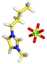
• For information about PDB foramt, please refer to documentation on RCSB website.
• We have the files in the folder at beginning:
  

  Filename Description bmi.pdb The anion structure data file in PDB format pf6.pdb The cation structure data file in PDB format modar or: modar.exe (forWindows) The primary Modar executable binary movar The structure visulalization tool viewene or: viewene.exe (forWindows) The utility for viewing the energies profile generated by modar top_all27_prot_na.rtf The residues’ topologies file of CHARMM force field par_all27_prot_na.prm The parameter files of CHARMM force field bmi.top pft.top The ions topology in CHARMM force field format bmi.prm pft.prm CHARMM force field parameters for the ions Waterbox.msf The small water box built in Example

  
  

 Step 1.  Build a ions pair by command:       

./modar step1_build_pair.inp

./modar step1_build_pair.inp  mol1=bmi.pdb mol2=pf6.pdb dis=6.0 nstep=500

• Let's take a glance to the script file "step1_build_pair.inp"
  

  if(!-var mol1)  getvar mol1  msg="no mol1 specified" chkfile=true if(!-var mol2)  getvar mol2  msg="no mol2 specified" chkfile=true if(!-var dis)   getvar dis   msg="no displacement distance specified" \                              default=6.0 min=1.0 max=20.0 if(!-var nstep) getvar nstep msg="how may cycles for energy minimiztion" \                              default=500 min=10  max=1000   #load force field include "loadff.inc"   #load first molecule loadmsf fmt="pdb" file=$mol1 build=false   #reset iseq of first molecule to 1 atom iseq newiseq=1 select="all"   tell natom select="all" natom1=$natom   #load the other molecule loadmsf fmt="pdb" file=$mol2 append=true build=false #reset iseq of first molecule to 2 atom iseq newiseq=2 select="iatom >=$natom1"   #change segment name to "ILC" atom segn newname="ILC" select="all"   #build topology build top   #replace molecules and separated somehow atom transto pos=(0,0,0) select="iseq 1" atom transto pos=($dis,0,0) select="iseq 2"   #add a restrain to pack a closed pair restrain dist k=100 refvalue=3 select="iseq 1" select="iseq 2"   #do minimization for the single molecule domin type=sd nstep=$nstep nprint=10 ftol=1e-5   #remove restraint restrain clear   #save msf and pdb savemsf file="step1_pair.msf" savecrd fmt=pdb file="step1_pair.pdb"

  where, we load the the anion and cation first and then describe the ions in CHARMM forcefiled; and then we use command "atom" to translate the ions, and then a displacement restraint is applied to the ionic pair, finally we do a short energy minimization to refine the position of ionic pair.
• The output files will be
  

  Filename File Type Description step1_build_pair.log Text The log message produced by Modar step1_pair.msf Text Ions pair structure file in Modar format with interpretation by FF given step1_pair.pdb Text Ions pair structure file in RCSB PDB format

 Step 2. Generate a box by replication from the single pair by command:

./modar step2_genbox.inp msf=step1_pair.msf  density=1.08 a=30

        The script used here is the same as the one used in the step2 of Example 1. The only difference is the feeding in MSF, density, box length, and no argument “rotate=true” needed.

• Please read the scipt file "step2_genbox.inp" for more details about these options.
• The output files will be:
  

  Filename File Type Description step2_genbox.log Text The log message produced by Modar, please read it and the input script if you are fresh to Modar, it may help a lot to understand how Modar works. step2_solvbox.msf Text Molecular structure file in Modar format with interpretation by FF given step2_solvbox.pdb Text Molecular structure file in RCSB PDB format step2_solvbox.ene Binary The energies profile of energy minimization pbc.inc Text PBC information for further MD simulation

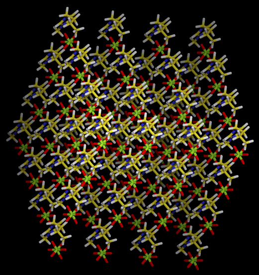
• Right now we have a “pseudo-solid” ions box with 250 pairs ions, the box size is 30x30x30; next we’ll melt it at 500K for 1ns MD simulation.
  

   

 Step 3. Melt the small box by command:

./modar step3_melt.inp nstep=500000

• Please read the scipt file "step3_melt.inp" for more details.
• The output files will be:
  

  Filename File Type Description step3_melting.log Text The log file step3_melting.trj Binary Trajectory in Movar binary format step3_melting.rst Binary The MD system state for resuming run step3_melting.rst.prev Binary The “backup” of last “rst” file, Modar make a backup for old restarting state when writing a new state for restarting run to deal some accidents like the storage run out off capacity. step3_melting.ene Binary The energies profile of MD simulation

  
  

 Step 4. Equlibrate the small box at room temperature by command:

./modar step4_equil_nvt.inp nstep=1000000 

• Please read the scipt file "step4_equil.inp" for more details.
• The output files will be:
  

  Filename File Type Description step4_equil_nvt.log Text The log file step4_annealing.trj Binary Trajectory fie in Movar format on annealing stage step4_ annealing.rst Binary The MD system state for resuming run step4_annealing.ene Binary The energies profile on annealing stage step4_equil_nvt.trj Binary Trajectory file on equilibration stage step4_equil_nvt.rst Binary The MD system state for resuming run step4_equil_nvt.ene Binary The energies profile on equilibration state

• please view the trajectory by command
  

  ./movar step2_solvbox.pdb step4_equil_nvt.trj

• Here is a snap shot of final state by movar
  
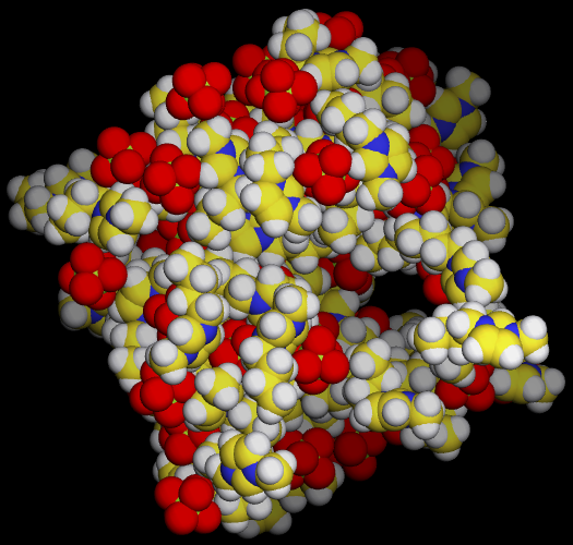
• As shown in the picture, there are some cavities in the system, since we initiated a wrong density in begining. So we need to do a NPT equilibration to get a correct density.
  

 Step 4.1. Equlibrate under NPT ensemble by command:

./modar step4.1_equil_npt.inp nstep=1000000 

• Please read the scipt file "step4.1_equil_npt.inp" for more details.
• The output files will be:
  

  Filename File Type Description step4_equil_npt.log Text The log file step4_equil_npt.trj Binary Trajectory file on equilibration stage step4_equil_npt.ene Binary The energies profile on equilibration state step4_equil_npt.rst Binary The MD system state for resuming run step4_equil_npt.msf Text The final structure in Modar MSF format step4_equil_npt.pdb Text The final structure in PDB format

• Please view the trajectory by command
  

  ./movar step2_solvbox.pdb step4_equil_npt.trj

• There is no cavity anymore.
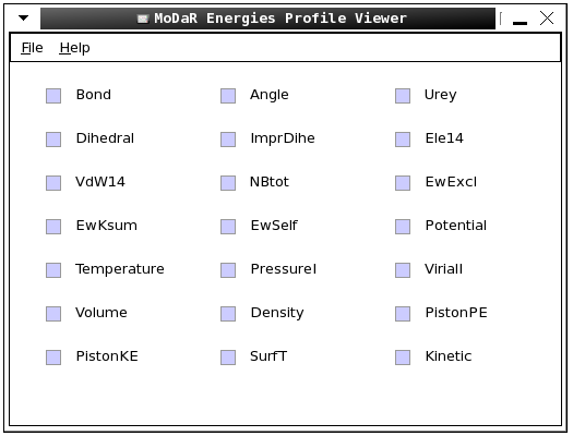
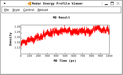
• Please view the energy profile by command
  

  ./viewene step4_equil_npt.ene

  As shown in bellow figure, the system reached the real density at about 500ps.
  
  

 Step 4.2. Calculate the radial distribution function by command:

./modar step4.2_calc_rdf.inp 

• We do this calculation to make sure the system is equlibrated enough.
• Please read the scipt file "step4.2_calc_rdf.inp" for more details.
• The ions pair RDF will be saved to file “rdf_bmi_pf6.txt”.
  
• Here is the result should be.
  

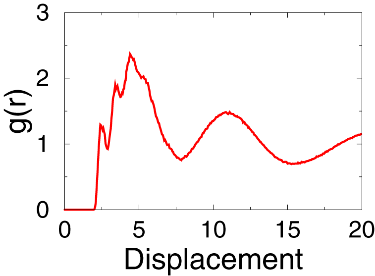
  As indicated by the picture, apparently the electrostatic interaction contribution is very significent in ionic liquid simulation.

  
  

 Step 5. Build a larger box by replicating from the small box by command:

./modar step5_gen_large_box.inp boxtype=cubic a=48  b=48 c=48

Or by following command to generate a cubic box with 500 pairs ions, and the size of box will be determined automatically.

• Please read the scipt file "step5_gen_large_box.inp" for more details.
  
• The output files will be:
  

  ./modar step5_gen_large_box.inp npair=250

 Step 6. Equlibrate the larger box at room temperature by command:

./modar -nobak step6_equil_nvt.inp nstep=5000

• In this step, we’ll heatup the system to 300K and run a short NVT equilibration.
• Please read the explanation of the scipt file "step6_equil_nvt.inp" for more details.
  
• The output files will be:
  

  Filename File Type Description step6_equil_nvt.log Text The log message produced by Modar step6_heatup.trj Binary The trajectory file in Modar format for heating up progress step6_heatup.ene Binary The energy profile of the heating up progress step6_heatup.rst Binary The system state for further simulation step6_equil_nvt.trj Binary The trajectory file in Modar format for heating up progress step6_equil_nvt.ene Binary The energy profile of the heating up progress step6_equil_nvt.rst Binary The system state for further simulation

  
  

 Step 6.1. Run a short NPT equilibration by command:

./modar -nobak step6.1_equil_npt.inp nstep=5000

• Please read the explanation of the scipt file "step6.1_equil_npt.inp" for more details.
  
• The output files will be:
  

  Filename File Type Description step6.1_equil_nvt.log Text The log message produced by Modar step6_equil_npt.trj Binary The trajectory file in Modar format for heating up progress step6_equil_npt.ene Binary The energy profile of the heating up progress step6_equil_npt.rst Binary The system state for further simulation step6_equil_npt.msf Text The final structure in Modar MSF format step6_equil_npt.pdb Text The final structure in PDB format

  
  

 Step 7. Add a water phase by command:

./modar -nobak step7.1_gen_water_box.inp 

./modar -nobak step7.2_merge.inp 

• In this step, we’ll add a water phase to the system.

• Please read the explanation of the scipt file "step7.1_gen_water_box.inp" and "step7.2_merge.inp" for more details.
  
• The output files will be:
  

  Filename File Type Description step7_add_water.log Text The log message produced by Modar step7_waterbox.mds Text   step7_waterbox.pdb Text   step7_two_phases.mds Text The whole MD system steup in Modar MDS format file step7_two_phases.pdb Text The whole MD system structure in RCSB PDB format file step7_two_phases.msf Text The final structure in Modar MSF format

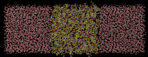
• Please visualize the system by command:
  

  ./movar step7_two_phases.pdb

  Here is the system look like.
  
  

 Step 8. Equilibrate the sytem with boundary restraint by command:

./modar -nobak step8_equil_npt.inp nstep=5000

• Please read the explanation of the scipt file "step8_equil_npt.inp" for more details.
• As shown in the input script file, we added two restraints term to maintain a interface between the two phases.
      "restrain zRange" to restrict the ions walking to the water phase;
      "restrain zBlock"  to block the water moving to the ionic phase;
  
• The output files will be:
  

  Filename File Type Description step8_equil_npt.log Text The log message produced by Modar step8_equil_npt.mds Text The whole MD system structure in Modar MSF format file step8_equil_npt.trj Binary The trajectory file in Modar format for the progress step8_equil_npt.ene Binary The energy profile of the progress step8_equil_npt.rst Binary The system state for further simulation

• Please view the energy profiles by command:
  

  ./viewene step8_equil_npt.ene There is a extra energy term, "RestraintEe", which is the restraint energy.

• Please view the trajectory by command:
  

  ./movar step7_two_phases.pdb step8_equil_npt.trj It should show a quick meshing event on the phase boundary.

  
  

 Step 9. Simulate the phases meshing process by command:

./modar step9_meshing.inp nstep=500000

./modar step9_meshing.mds nstep=500000

• Please read the explanation of the scipt file "step9_meshing.inp" for more details.
  
• The output files will be:
  

  Filename File Type Description step9_meshing.log Text The log message produced by Modar step9_meshing.mds Text The whole MD system steup in Modar MDS format file step9_meshing.trj Binary The trajectory file in Modar format for the progress step9_meshing.ene Binary The energy profile of the progress step9_meshing.rst Binary The system state for further simulation

• Please view the energy profiles by command:
  

  ./viewene step9_meshing.ene

  
  

 Step 10. Result analysis by command:

./modar ana.inp

• Please read the scipt file "ana.inp" for more details.
• The output files will be:
  

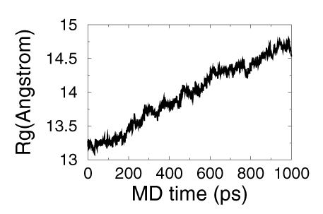
  Filename File Type Description zrgy.txt Text The profile of radius of gyration of ionic liquid (only Z component) aout.txt Text How many anion moved to the water with the time going cout.txt Text How many cation moved to the water with the time going

  
  
• Here we use the changing of radius of gyration of the ionic liquid as the measurement of the meshing process.
  
• Here is the how many number of cation and anion moved to the water with the time going
  I cannot draw a solid conculation since I don't have enough samples yet. However, it does show us that this ionic liquid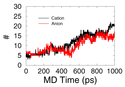

 Summary

• In this practice, we built a ionic liquid solvent from scratch, then we add water to the system to create a two phase system, then the meshing process between the ionic liquid and water was simulated.
  

 Computational detail

• The MD system was modeled in CHARMM 27 force field.
• Berendsen weak temperature coupling method were used for tempering process.
• Nose-Hoover thermostat approach was used for keeping constant temperature in NVT and NPT equilibrating simulations, the Langevin piston approach was used for constant pressure coupling.
• Shake constraint method was applied for all hydrogen relatived bonds in all simulation.
• The long range electrostatic interactions were evaluated precisely through PME algorithm, and the short range interactions were truncated at 10.0 angstrom with a switch function.
• All simulations were propograted using leapfrog integrator with a time step 2fs, and samples were collected for every 1ps second.