Here is the procedures step-by-step

1. Describe the protein model by force field

2. Generate a water box

3. Add counter ions

4. Merge all

5. Do energy minimization

6. Heat up to 300K

7. Run a short NVT equilibration

8. Run a short NPT equilibration

9. Continue 2ns NPT equilibration

10. Heat up to 500K

11. Unfolding at 500K

12. Result analysis

  Preparations

• HP36 is composed of three helices (residues Asp44-Lys48, Arg55-Phe58 and Leu63-Lys70) which are packed together to share a hydrophobic core mainly contributed by the phenylalanine and leucine residues as shown in bellow figure. The three helices are connected by a loop (residues Ala49-Thr54) and a turn (residues Ala59 to Pro62) (McKnight, C. J., Matsudaira, P. T., and Kim, P. S. (1997) NMR structure of the 35-residue villin headpiece subdomain, Nature Structural Biology 4, 180-184). It’s known that HP36 folds on the microsecond timescale and is very thermostable. Its small size and rapid folding have made it an exceptionally popular model protein for theoretical and computational studies of protein folding and dynamics.
  
• We need an initial structure of the protein, which can be downloaded from RCSB protein data bank, go website http://www.pdb.org and search with keyword “villin headpiece”, then go entry “1VII” to download the PDB file.
• For information about PDB foramt, please refer to documentation on RCSB website.
• We have the files in the folder at beginning:
  

  Filename File Type Description 1VII.pdb Text The protein initial structure file (solved by NMR) downloaded form RCSB waterbox.msf Text A pre-build water solvent system in a cubic shape modar or: modar.exe (forWindows) executable The primary Modar executable binary viewene or: viewene.exe (forWindows) executable The utility for viewing the energies profile generated by modar step1_build_solute.inp script The Modar script for describing protein in FF step2_gen_solvbox.inp script for building a water box step3_add_ions.inp script for adding and placing contour ions step4_merge.inp script for putting protein and ions to the water box step5_minimize.inp script for optimizing the system by energy minimization step6_heatup.inp script for heating up the system to temperature desired Step7_equil_nvt.inp script for running a short equilibration with NVT condition step8_equil_npt.inp script for running a short equilibration with NPT condition step9_equil_npt_more.inp script for building a compact MD core for further long scale time simulation step10_heat_to_500k.inp Script For heating to 500K step11_unfolding.inp Script Unfolding calc_rmsd.inp Script For RMSD profile analysis calc_rmsd2.inp Script For unfolding pathway analysis do_pdb_nomination_replacement.inc Script For PDB to Modar nomination replacement do_protein_dna_rna_terminals_patch.inc Script For protein, RNA, DNA terminus patching loadff.inc Script Load Charmm force field nptc.inc Script NPT ensemble setup with Nose-Hoover Thermostat and Langevin Piston pressure coulpling

  
  

 Step 1.  Describe the protein in CHARMM force field by command:       

./modar step1_build_solute.inp

./modar step1_build_solute.inp pdb=1VII.pdb

• Please read the scipt file "step1_build_solute.inp" for more details. This script file is general template for interprelating protein, RNA and DNA. Please read the comments (in green) first before doing a practice and pay attension to the lines marked in red color.
• The output files will be
  

  Filename File Type Description step1_build_solute.log Text The log message produced by Modar step1_solute.msf Text Solute structure file in Modar format described in FF given step1_solute.pdb Text Solute structure file in RCSB PDB format solute_size.inc Text The extension of solute in Modar assign statement

• Some log message would be printed on screen (step1_osl.html)

 Step 2. Generate a water box by command:

./modar step2_gen_solvent_box.inp type=cubic a=60

        Or without argument “boxtype=cubic a=60”, it will ask you for box type and a,b,c respectively.

• Please read the scipt file "step2_gen_solvent_box.inp" for more details about these options.
• The output files will be:
  

  Filename File Type Description step2_gen_solvent_box.log Text The log message produced by Modar step2_solvbox.msf Text The solvent structure file in Modar format described in FF given step2_solvbox.pdb Text Solvent structure file in RCSB PDB format pbc.inc Text The PBC setup for further usage

   

 Step 3. Add counter ions by command:

./modar step3_add_ions.inp method=hybrid ionc=0.1

• Please read the scipt file "step3_add_ions.inp" for more details.
• The output files will be:
  

  Filename File Type Description step3_add_ions.log Text The log message produced by Modar step3_with_ions.msf Text Solute with ions structure file in Modar format described in FF given step3_with_ions.pdb Text Solute with ions structure file in RCSB PDB format

• Some log message would be printed on screen (step2_osl.html).

  
  

 Step 4. Put solute and salt to the water box by command:

./modar step4_merge_all.inp 

• Please read the scipt file "step4_merge_all.inp" for more details. This scrip file could serve as tempelate script for merging several MSF file together.
• The output files will be:
  

  Filename File Type Description step4_merge_all.log Text The log message produced by Modar step4_all.msf Text The whole MD system structure in Modar MSF format file step4_all.pdb Text The whole MD system structure in RCSB PDB format file

• Some log message would be printed on screen (step4_osl.html).

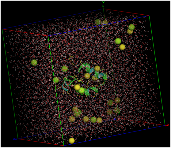
• Please view the system by command:
  

  ./movar step4_all.pdb

• Here is the whole MD system snaped by Movar
  
  

 Step 5. Do a serial of energy minimization by command:

./modar step5_do_minimization.inp nstep1=200 nstep2=200 nstep3=200 nstep4=200 

• Please read the scipt file "step5_do_minimization.inp" for more details.
• The output files will be:
  

  Filename File Type Description step5_do_minimization.log Text The log message produced by Modar step5_minimized.msf Text The whole MD system structure minimized in Modar MSF format file step5_minimized.pdb Text The whole MD system structure minimized in RCSB PDB format file step5_min?.trj Binary The trajectory file in Modar format for every minimization stage respectively step5_min?.ene Binary The energy profile for every minimization state respectively, and it can be viewed by tool “viewene” miniport.txt Text 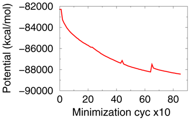The potential energy profile extracted from the log file for the whole minimization progress.

• Plot the file “miniport.txt” should get a picture as shown bellow.

  
  

 Step 6. Heatup the system by command:

./modar -nobak step6_heatup.inp nstep=2500 ttar=300  tinit=50 rand=false

• Please read the scipt file "step6_heatup.inp" for more details.
• The output files would be:
  

  Filename File Type Description step6_heatup.log Text The log message produced by Modar step6_heatup.mds Text The whole MD system steup in Modar MDS format file step6_heatup.pdb Text The whole MD system structure heatuped in RCSB PDB format file step6_heatup.trj Binary The trajectory file in Modar format for heating up progress step6_heatup.ene Binary The energy profile of the heating up progress step6_heatup.rst Binary The system state for further simulation

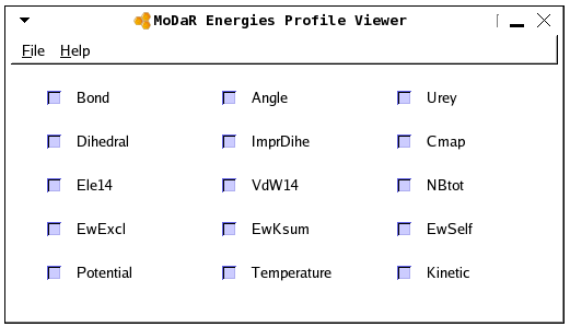
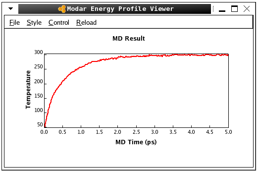
• Please check the energy profile by command:
  

  ./viewene step6_heatup.ene As shown in bellow pictures, the system has been tempering from 50K to 300K gradually.

  
  
  
  

 Step 7. Run a short NVT equilibration by command:

./modar -nobak step7_equil_nvt.inp nstep=2500

• Please read the scipt file "step7_equil_nvt.inp" for more details.
  
• The output files will be:
  

  Filename File Type Description step7_equil_nvt.log Text The log message produced by Modar step7_equil_nvt.mds Text The whole MD system steup in Modar MDS format file step7_equil_nvt.pdb Text The whole MD system structure in RCSB PDB format file step7_equil_nvt.trj Binary The trajectory file in Modar format for equilibrating progress step7_equil_nvt.ene Binary The energy profile of the equilibrating progress step7_equil_nvt.rst Binary The system state for further simulation

• Please check the energy profile by command
  

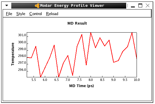
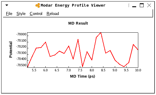
  ./viewene step7_equil_nvt.ene The poteintial and temperature fluctuation would be something as shown in bellow picture.

  
  

 Step 8. Run a short NPT equillibration by command:

./modar -nobak step8_equil_npt.inp nstep=2500

• Please read the explanation of the scipt file "step8_equil_npt.inp" for more details.
  
• The output files will be:
  

  Filename File Type Description step8_equil_npt.log Text The log message produced by Modar step8_equil_npt.mds Text The whole MD system structure in Modar MSF format file step8_equil_npt.pdb Text The whole MD system structure in RCSB PDB format file step8_equil_npt.trj Binary The trajectory file in Modar format for the progress step8_equil_npt.ene Binary The energy profile of the progress step8_equil_npt.rst Binary The system state for further simulation

  
  

 Step 9. Resume a 2ns NPT  equilibration by command:

./modar step9_equil_npt_more.inp nstep=1000000

Or we could set argument “nstep=0” to build the MD core only, then submit job to compute node to run job by command:

./modar step9_equil_npt_more.mds nstep=1000000

• Please read the explanation of the scipt file "step9_equil_npt_more.inp" for more details.
  
• The output files will be:
  

  Filename File Type Description step9_equil_npt_more.log Text The log message produced by Modar step9_equil_npt_more.mds Text The whole MD system steup in Modar MDS format file step9_equil_npt_more.trj Binary The trajectory file in Modar format for the progress step9_equil_npt_more.ene Binary The energy profile of the progress step9_equil_npt_more.rst Binary The system state for further simulation

  
  

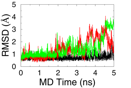
 Step 9.1. Calculate the RMSD profile by command:

./modar calc_rmsd.inp msf=step6_heatup.msf \  
           mds=step9_equil_npt_more.mds \
           pdb=step5_minimized.pdb \
           trj=step9_equil_npt_more.trj

• In this step, we’ll add a water phase to the system.

• Please read the explanation of the scipt file "calc_rmsd.inp" for more details.
  
• The output files will be:
  

  Filename File Type Description rmsd.txt Text The overall RMSD bbrmsd.txt Text The backbone RMSD

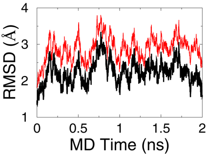
• The backbone RMSD fluctaion should be similar to the bellow picture, the backbone RMSD is in black, and the overall RMSD is in red.

  
  

 Step 10. Heaup the system to 500K under NVT condition,
                then do a short NVT equilibration and also a short NTP equilibration

                by command:

./modar step10_heat_to500k.inp

• Please read the explanation of the scipt file "step10_heat_to500k.inp" for more details.
• The output files will be:
  

  Filename File Type Description step10_heat_to400k.trj step10_equil_nvt.trj step10_equil_npt.trj Binary The trajectory file in Modar format for the progress step10_heat_to400k.ene step10_equil_nvt.ene step10_equil_npt.ene Binary The energy profile of the progress step10_heat_to400k.rst step10_equil_nvt.ene step10_equil_npt.ene Binary The system state for further simulation step10_equil_npt.mds Binary The whole MD system steup in Modar MDS format file

  
  

 Step 11.   Continue for 10 ns NPT simulation to unfolder the protein by command:

./modar step11_unfolding.inp nstep=2500000

./modar step11_unfolding.mds nstepmore=2500000

• Please read the explanation of the scipt file "step11_unfolding.inp" for more details.
  
• The output files will be:
  

  Filename File Type Description step11_unfolding.trj Binary The trajectory file in Modar format for the progress step11_unfolding.ene Binary The energy profile of the progress step11_unfolding.rst Binary The system state for further simulation step11_unfolding.log Binary The log file

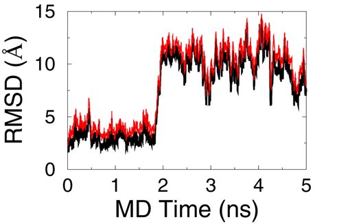
•  The RMSD profile can be computed using the same script “calc_rmsd.inp” used in step9 by command.
  

  ./modar calc_rmsd.inp msf=step6_heatup.msf \ mds=step9_equil_npt_more.mds \ pdb=step5_minimized.pdb \ trj=step10_unfolding.trj

  The RMSD profile in my simulation:
  

  
  

 Step 12. Unfolding pathway analysis by command:

./modar calc_rmsd2.inp msf=step6_heatup.msf  \
              mds=step9_equil_npt_more.mds \
              pdb=step5_minimized.pdb \
              trj=step10_unfolding.trj

• Please read the scipt file "calc_rmsd2.inp" for more details.
• The output files will be:
  

  Filename Description bbrmsd_h1.txt backbone RMSD profile of Helix 1 (seq 43:51) bbrmsd_h2.txt backbone RMSD profile of Helix 2 (seq 54:61) bbrmsd_h3.txt backbone RMSD profile of Helix 3 (seq 62:73) bbrmsd_h12.txt backbone RMSD profile of Helix 1&2 (seq 43:61) bbrmsd_h23.txt backbone RMSD profile of Helix 2&3 (seq 54:73)

  
  
• Bellow is the plot of file “bbrmsd_h1.txt”, “bbrmsd_h2.txt”, “bbrmsd_h3.txt”.
  
• Bellow is the plots of file “bbrmsd_h12.txt” and “bbrmsd_h23.txt”
  Obviously, the unfolding pathway for my simulation is: the turn between Helix 2 and Helix 3 opened first, and then helix 2 and 3 opened respectively, the N-terminal helix is the most stable part.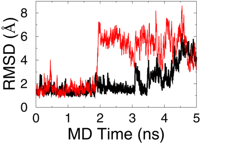

 Summary

• In this example, we practise a protein simulation in a explicit water solvent, the system was equilibrated 2ns at room temperature under NPT ensemble, then the unfolding pathway was investigated through the NPT equilibrating simulation at high temperature 500K.
  

 Computational detail

• The MD system was modeled in CHARMM 27 force field.
• Berendsen weak temperature coupling method were used for tempering process.
• Nose-Hoover thermostat approach was used for keeping constant temperature in NVT and NPT equilibrating simulations, the Langevin piston approach was used for constant pressure coupling.
• Shake constraint method was applied for all hydrogen relatived bonds in all simulation.
• The long range electrostatic interactions were evaluated precisely through PME algorithm, and the short range interactions were truncated at 10.0 angstrom with a switch function.
• All simulations were propograted using leapfrog integrator with a time step 2fs, and samples were collected for every 1ps second.