Here is the procedures step-by-step

1. Describe a single chlorine anion in CHARMM force field

2. Generate a water box by replicating from the small box built in Example 1

3. Add more ions by MC approach

4. Put ions in to the water box

5. Energy minimization

6. Heatup the system

7. Run a short NVT equilibration

8. Run a short NPT equilibration

9. Continue 5ns more NPT simulation to collect samples for RDF evaluation

10. Derive the PMF through RDF calculation

  Preparations

• We need to start from a single chlorine ion in a PDB format file as shown bellow.
  

  ATOM      1  CLA CLA     1       0.000   0.000   0.000

• For information about PDB foramt, please refer to documentation on RCSB website.
• So let’s make a folder, say “kcl_pmf”, and create a text file “cl.pdb” with above contents, and copy Modar executable binaries, CHARMM force field files and the water box build in Example 1.
• We have the files in the folder at beginning:
  

  Filename File Type Description cl.pdb Text The single chlorine anion in PDB format waterbox.msf Text The small water box generated in Example 1 modar or: modar.exe (forWindows) Executable binary The primary Modar executable binary viewene or: viewene.exe (forWindows) Executable binary The utility for viewing the energies profile generated by modar top_all27_prot_na.rtf Text The residues’ topologies file of CHARMM force field par_all27_prot_na.prm Text The parameter files of CHARMM force field

  
  

 Step 1.  Describe the single chlorine anion in CHARMM FF by following command       

./modar step1_build_solute.inp

            where, "modar" is the primary binary of Modar package,

                         "step1_build_solute.inp" is the script file in Modar script language,                 

• Let's take a glance to the script file "step1_single_opt.inp"
  

  #load force field loadfftop fmt=chm file="top_all27_prot_na.rtf" loadffprm fmt=chm file="par_all27_prot_na.prm"   #load molecule structure file loadmsf fmt="pdb" file="cl.pdb"   #replace the atom name "CL-" to "CLA" which used in CHARMM force field atom name newname="CLA" select="all"   #replace the resdiue name "CL-" to "CLA" which used in CHARMM force field atom resname newname="CLA" select="all"   #assign a segment name atom segname newname="ION" select="all"   #build and describe the molecule according to the force field build top   #save msf and pdb savemsf file="step1_single.msf" savecrd fmt=pdb file="step1_single.pdb"

  where, we use command "loadfftop" and "loadffprm" to load CHARMM 27 force field first; then loaded the the single chlorine ion by command "loadmsf"; then we call "atom" command to do some nomination modification; then we call "build" command to describe the ion in CHARMM forcefiled; finally we use command "savemsf" to store the structure to Modar "msf" format file, and also save a PDB format file.
• The output files will be
  

  Filename File Type Description step1_build_solute.log Text The log message produced by Moda step1_single.msf Text Molecular structure file in Modar format with interpretation in force field given step1_single.pdb Text Molecular structure file in RCSB PDB format

 Step 2. Generate a box by replication from the small water box created in Example 1
              by command:

./modar step2_gen_solvent_box.inp

          It will prompt user interactive message for the type and the size of box, press enter here to use the default value, here we'll try the truncated octahidralt box which will same some computation cost, the size of 48 Angstrom is good for this instance.

         Or by follow command without interactive prompt.

./modar step2_gen_solvent_box type=octa a=48

• Please read the scipt file "step2_gen_solvent_box.inp" for more details about these options.
• The output files will be:
  

  Filename File Type Description step2_gen_solvent_box.log Text The log message produced by Modar, please read it and the input script if you are fresh to Modar, it may help a lot to understand how Modar works. step2_solvbox.msf Text Molecular structure file in Modar format with interpretation by FF given step2_solvbox.pdb Text Molecular structure file in RCSB PDB format pbc.inc Text PBC information for further MD simulation

  
  

 Step 3. Add more ions by command:

./modar step3_add_ions.inp

• Please read the scipt file "step3_add_ions.inp" for more details.
• The output files will be:
  

  Filename File Type Description step3_add_ions.log Text The log message produced by Moda step3_with_ions.msf Text The ions structure in Modar format with interpretation by FF given step3_with_ions.pdb Text The ions structure in RCSB PDB format

  
  

 Step 3. Put ions into the water box by command:

./modar step4_merge_all.inp 

• We have the water box in step 2 and the ions distribution in step 3; in this step, it shows user how to solvate the ions to the water by merging the two “MSF” together and removing the water molecules which overlaps or have bad contacts with the ions simply.
  

• Please read the scipt file "step4_merge_all.inp" for more details. It is actually a template for merging two or more parts of MD system together.
• The output files will be:
  

  Filename File Type Description step4_merge_all.log Text The log message produced by Modar step4_all.msf Text The whole system in Modar format with interpretation by FF given step4_all.pdb Text The whole sytem in RCSB PDB format file

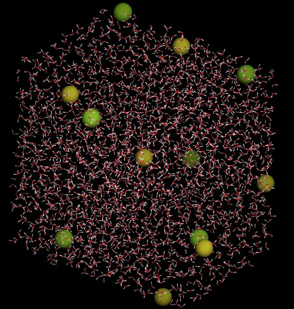
• please view the MD system build by command
  

  ./movar step4_all.pdb

• Here is a snap shot by movar
  
  

 Step 5. Do a energy minimization by command:

./modar step5_do_minimization.inp 

• In this step we’ll do a short energy minimization since the system may still have some bad contacts.
• Please read the explanation of the scipt file "step5_do_minimization.inp" for more details.
  
• The output files will be:
  

  Filename File Type Description step5_do_minimization.log Text The log message produced by Modar step5_minimized.msf Text The whole MD system structure minimized in Modar MSF format file step5_minimized.pdb Text The whole MD system structure minimized in RCSB PDB format file min?.trj Binary The trajectory file in Modar format for every minimization stage respectively min?.ene Binary The energy profile for every minimization state respectively, and it can be viewed by tool “viewene” miniport.txt Text The potential energy profile extracted from the log file for the whole minimization progress.

• Plot the miniport.txt by xmgr or gnuplot, it should show that the total potential of system is decreased speedly in beginning.

• Or view the energy profiles by command:
  

  ./viewene min1.ene

 Step 6. Heatup the system by command:

./modar -nobak step6_heatup.inp nstep=2500 Ttar=300  Tinit=50 rand=false

• In this step, we’ll heatup the system to 300K through Berendsen thermostat approach and equilibrate the system somehow.
• Please read the explanation of the scipt file "step6_heatup.inp" for more details.
  
• The output files will be:
  

  Filename File Type Description step6_heatup.log Text The log message produced by Modar step6_heatup.mds Text The whole MD system steup in Modar MDS format file step6_heatup.pdb Text The whole MD system structure heatuped in RCSB PDB format file step6_heatup.trj Binary The trajectory file in Modar format for heating up progress step6_heatup.ene Binary The energy profile of the heating up progress step6_heatup.rst Binary The system state for further simulation

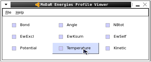
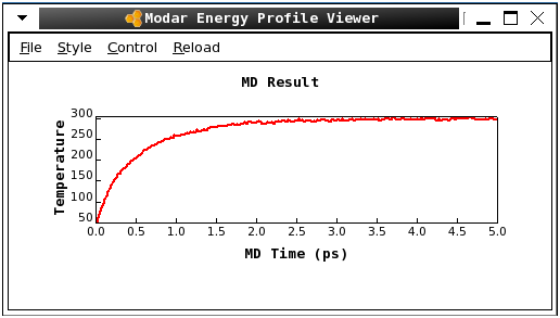
• Please view the energy profiles by command:
  

  ./viewene step6_heatup.ene

  As shown in bellow pictures, the system has been tempering from 50K to 300K gradually.
  
  

 Step 7. Run a short NVT equilibration by command:

./modar -nobak step7_equil_nvt.inp nstep=2500

• In this step, we’ll equilibrate the system under NVT condition with Nose-Hoover thermostat method.

• Please read the explanation of the scipt file "step7_equil_nvt.inp" for more details.
  
• The output files will be:
  

  Filename File Type Description step7_equil_nvt.log Text The log message produced by Modar step7_equil_nvt.mds Text The whole MD system steup in Modar MDS format file step7_equil_nvt.pdb Text The whole MD system structure in RCSB PDB format file step7_equil_nvt.trj Binary The trajectory file in Modar format for equilibrating progress step7_equil_nvt.ene Binary The energy profile of the equilibrating progress step7_equil_nvt.rst Binary The system state for further simulation

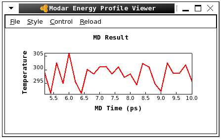
• Please view the energy profiles by command:
  

  ./viewene step7_equil_nvt.ene

  Here is a screen shot of the fluctation of temperature.
  
  

 Step 8. Run a short NPT equilibration by command:

./modar -nobak step8_equil_npt.inp nstep=5000

• In this step, we’ll run a short NPT equilibration with Nose-Hoover thermostat for temperature control and Langevin piston method for pressure coupling. Bellow is the content of script file “step8_equil_npt.inp” to do the equilibration.

• Please read the explanation of the scipt file "step8_equil_npt.inp" for more details.
  
• The output files will be:
  

  Filename File Type Description step8_equil_npt.log Text The log message produced by Modar step8_equil_npt.mds Text The whole MD system structure in Modar MSF format file step8_equil_npt.pdb Text The whole MD system structure in RCSB PDB format file step8_equil_npt.trj Binary The trajectory file in Modar format for the progress step8_equil_npt.ene Binary The energy profile of the progress step8_equil_npt.rst Binary The system state for further simulation

• Please view the energy profiles by command:
  

  ./viewene step8_equil_npt.ene

  
  

 Step 9. Continue 5ns more NPT simulation by command:

./modar step9_equil_npt_more.inp nstep=2500000

./modar step9_equil_npt_more.mds nstep=2500000

• We’ll continue the NPT simulation for 5ns more to collect enough samples for PMF evaluation.

• Please read the explanation of the scipt file "step9_equil_npt_more.inp" for more details.
  
• The output files will be:
  

  Filename File Type Description step9_equil_npt_more.log Text The log message produced by Modar step9_equil_npt_more.mds Text The whole MD system steup in Modar MDS format file step9_equil_npt_more.trj Binary The trajectory file in Modar format for the progress step9_equil_npt_more.ene Binary The energy profile of the progress step9_equil_npt_more.rst Binary The system state for further simulation

• Please view the energy profiles by command:
  

  ./viewene step9_equil_npt_more.ene

  
  

 Step 10. Calculate the radial distribution function by command:

./modar rdf.inp

• Please read the explanation of the scipt file "rdf.inp" for more details.
  
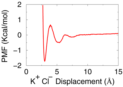
• The output file will be “rdf_K_CL.txt” which is the radial distribution function of K-CL ions pair, the displacement PMF of the ions pairs can be derived simply by following awk command
  

  awk '{ if($2>0) print $1,-0.6*log($2) }' rdf_K_CL.txt > pmf_K_CL.txt

  Plot the file "pmf_K_CL.txt", the PMF should be identical to bellow figure.
  

 Summary

• In this practice, we generated a truncated octahidralt water box by replicating from the small water box built in Example 1, then we put 0.1M KCL salt to box; then the system was tempered to 300K and undergoed a short NVT equilibration, and also a short NPT equilibration; finally total 5ns second NPT samples were collected for radial distribution function (RDF) evaluation, and displacement PMF of ions pairs was derived.
  

 Computational detail

• The MD system was modeled in CHARMM 27 force field.
• Berendsen weak temperature coupling method were used for tempering process.
• Nose-Hoover thermostat approach was used for keeping constant temperature in NVT and NPT equilibrating simulations, the Langevin piston approach was used for constant pressure coupling.
• Shake constraint method was applied for all hydrogen relatived bonds in all simulation.
• The long range electrostatic interactions were evaluated precisely through PME algorithm, and the short range interactions were truncated at 10.0 angstrom with a switch function.
• All simulations were propograted using leapfrog integrator with a time step 2fs, and samples were collected for every 1ps second.